ABIC

summary

Formula

forward modeling:

• j: station index.
• q: slip component, along strike and dip direction.
• integration in space : $ \int_s ~d\xi $
• integration in time : convolution operator *

suppose:

• $ X_k $ : basis functions for space.
• $ T_l $ : basis functions for time
• $ t_k $ : arrival time of rupture front at grid k.
• Note : we just convert to estimating $ a_{qkl} $ there is no need to be orthogonal basis, here adopt Bézier basis functions. so the shape can be control by neibourhood grid which favor applying smoothing constrians.

with

$X_k$ is analytical expression, but $g_{qkj}$ is not. so there still exist error raised from the discretization

if Consider uncertain of Green Function then:

apply filter $B(t)$

Propagation of uncertainty

variance-covariance matrix

Discrete convolution

Bézier curve

recursion formula

General form of a NURBS surface

A NURBS surface is obtained as the tensor product of two NURBS curves, thus using two independent parameters u and v (with indices i and j respectively):

with

as rational basis functions.

simple introduction of Bayesian rule

Joint probability of two events A and B:

In Bayesian probablity theory: one “events” is Hypothesis. the other is Data. so:

• $P\left(D|H\right)$: likelihood function, as it assesses the probablity of the observed data arising from hypothesis.
• $P\left(H\right)$: prior, as it reflects one′ prior knowledge before the data are considered.
• $P\left(H|D\right)$: Posterior, as its name suggests. reflects the probability of the hypothesis after consideration.

A simple example

let′s say we have some quantity in the world, $x$, and our observation of this quantity,$y$, is corrupted by additive Gaussian noise, e:

• we might want to pick the value of $x$ that maximizes this distribution

• alternatively, we may want minimize the mean squared error of our guesses, then we should pick the mean of (Px|y);

let′s draw upon our existing knowledge. x with mean of 12,variance of 1. Thus,

The x which maximizes $P(x|y)$ is the same as that which minimizes the exponent in brackets which may be found by simple algebraic manipulation to be:

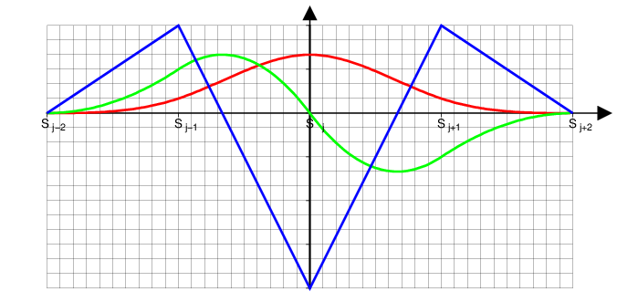
normalized bicubic B-splines

where

which $ M_{4,j}(s) $ is the B-spline function of order 4(degree 3)

value of center point

value of grid

integration of $M_{r,j}$

roughness

suppose coordinate on fault then $f_1=f_2=0, h_1=h_2=1$

M_4,i 积分，微分，最大值， M_4,j * M_4,j 积分微分

suppose: errors $e$ to be Gaussian with

$\sigma ^2 $ is unknow scale factor

likelihood function:

here $ || E || $ denotes the absolute value of the determinant of $ \mathbf{E} $

prior information:

posterior pdf

Marginal likelihood

Akaike Bayesian Information Criterion(ABIC)

with

for certain values of $\sigma ^2 $ and $\alpha ^2 $, minimizing $s(\mathbf{a}) $, $\frac{\partial s(\mathbf{a})}{\partial \mathbf{a}}=0 $

the solution is:

then, denoting

rewrite $s(\mathbf{a}) $

Gaussian integral Suppose A is a symmetric positive-definite (hence invertible) $n \times n$ covariance matrix. Then,

subsitute equation (9) into equation (4), carrying out the integration of marginal likelihood equation (3) (see gaussian integral eq.(10)).

then

substitute equation(12) into ABIC then rewrite.

Matrix Calculus

other notes and notions.

Consider a vector-valued function $\mathbb{R}^n\mapsto\mathbb{R}^m$ of order $m \times 1$, such that

The diferentiation of such a vector-valued function $\mathbf{F}(\mathbf{x})$ by another vector x of order $n\times1$ is ambiguous in the sense that the derivative

can either be expressed as an $m \times n$ matrix ( numerator layout convention ), or as an $n \times m$ matrix ( denominator layout convention ), such that we have

draft

• $ M_k \sim Length^{-1} $
• $ N_k \sim 1 ; \int N_k N_k~ds \sim Length ; \int \int N_k N_q~d\xi~d\xi=area $
• $ \int N_k~ds = \Delta s $
• $ \int M_k~ds = \frac{1}{n} $
• $ a_{kl} \sim Length $
• $ R_{jklpq} \sim Length^{-2} $
• $ r {\sim a^{T}} \mathbf{R} a \sim 1 $

STATIC DATA

if considering uncertain of Green Function( $\delta G $ ), then follows the same formulation derivation with seismic data.

roughness scheme

scheme 1: T.Yabuki(1992):

scheme 2: Yukitoshi Fukahata(2004)

Note:

• here omit slip-direction component.
• base function of time: triangle. so $r_2$ adopt first derivative
• the red part we adopt bilinear B-splines in $\xi_1$, $\xi_2$ direction, can be replace by scheme1.

scheme 3:

Yuji Yagi(2008)

Yuji Yagi(2011)

Note:

• here use second dirative for time, so the base funcion for time is also expressed by B-spine.

scheme

• both time and space base function represented by B-spine function with second order differentiability, (bilinear B-spine for space)
• apply $\int_T$ and $\int_\Sigma$ to abtain a scalar value.
• apply $[\cdots]^2$ to abtain this form: $\mathbf{a}^T\mathbf{G}\mathbf{a}$
• compare scheme 1,2 with 3: $ {\left[{\nabla}^2\dot{D}\right]}^{2} \iff \mathbf{a}^T\mathbf{G}\mathbf{a} \iff S^{T} S $
• conbine scheme 1,2,3 then: